What did the model actually see?

Summary
On our journey toward training on a trillion tokens, we have learned what matters. In this post we share how we build:
- A stable and efficient training framework. Enabling seamless training resumption after preemption or hardware failure, packing strategies to keep compute on real tokens, and end-to-end testing to catch regressions before they become expensive.
- Thorough data observability. We monitor what actually reaches the model, not just the recipe: the realized mixture and per-source statistics, collected live during the run.
- Trustworthy benchmarks. We don't take a score at face value: aggressive decontamination of the training data against every benchmark, and recording the generations behind a number.
Introduction
Building frontier agentic reasoning models for clinical work means training a generalist model to navigate clinical workflows end-to-end: reasoning over long patient records, calling diagnostic tools, navigating radiology viewers, scrolling through whole-slide pathology images, and connecting what it learns from those tools back to a clinical question. These are tools that off-the-shelf foundation models never see during training and are not natively calibrated to operate.
In a little over a year, we moved from training dense ~7B parameter multimodal vision-language models on a few hundred million tokens to 100B-token runs on 10-100x larger MoE models, with a roadmap toward trillion-token-scale continued pre-training (CPT). In our approach, the model architecture is treated as fixed. By benchmarking several open weight models that reported data sources and performances transparently, we settled on a strong base. This leaves the data as the primary variable we control in CPT and post-training. In what follows, we will therefore take a data-centric view on the stack that we’ve built.
The first decision is the mixture itself: a three-way tug-of-war between installing new clinical knowledge, retaining the base's general skills, and warming up its latent ones. The rest is the engineering that delivers that mixture at scale:
- a robust training framework for 100B+ MoE models that tracks not just training progress but the dynamics, hardware utilization, and data statistics of a run
- efficient data streaming to focus the compute where it matters
- observability to track down any failure and resume from a given state across data, model, and hardware (and to see what the model actually trained on)
- an evaluation signal we can trust: broadly mapping the performance landscape we care about and rigorously decontaminating the test data
Mid-training as a three-way tug-of-war
Rather than pre-training models from scratch, we start from capable models that have already been instruction-tuned and optimized for reasoning, and tool-use. We have previously verified that this yields stronger and better-performing models than starting from a checkpoint that was only pre-trained. However, a naïve continued pre-training on raw biomedical domain data would easily jeopardize the model’s learnt capabilities. To preserve these learnt skills, we craft a careful mix of raw, web-scale data (both text-only, image-captioning, and interleaved data), instruction-formatted Q&A and VQA, multi-turn conversations (with and without reasoning traces and images), as well as tool-use data. These instruction-formatted data components lean heavily on the general domain, while the raw, unformatted data is predominantly composed of domain-specific biomedical and clinical data intended to teach the model domain-specific knowledge. Technically, what we do is CPT, yet our data mixture moves this closer to what is often understood as mid-training, see e.g. in Liu et al. (2025)1. Conventional CPT would rely exclusively on in-domain data and is often accompanied by a sharp performance drop in orthogonal domains – something that we aim to prevent by carefully crafting a balanced data mix.
Thus, we view our CPT stage as a three-way tug-of-war between warmup, skill retention, and the target domain shift; see also PRISM2 for an in-depth analysis of the mid-training paradigm. Here we will briefly outline each of these directions:
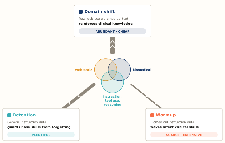
Mid-training as a tug-of-war between three data types, each defined by which two properties it combines. The circles are the properties (biomedical content, web-scale volume, instruction/tool-use/reasoning format); each data type sits in a pairwise overlap: domain shift (biomedical + web-scale) reinforces clinical knowledge, retention (web-scale + instruction) guards the base's general skills, warmup (biomedical + instruction) wakes latent clinical skills. Each pulls the mixture toward it with a force set by its abundance, so warmup, scarce and expensive to obtain, pulls with the thinnest rope. The triple overlap, representing web-scale biomedical instruction data, is not readily available and we reserve this for a future blog post on synthetic data generation for post-training.
The base model already has latent clinical core skills (instruction following, medical reasoning, basic tool-use), but calibrated for consumer-facing chatbots rather than assisting in professional clinical workflows. Warmup turns up the model's responsiveness on these skills by exposing it to clinical-shaped versions of them, e.g. reasoning traces injected into biomedical articles, or clinical VQA.
The second direction is retention: The base already knows English and a few other languages, math, code, and has some broad "world knowledge". We can't afford to erode any of that while chasing clinical capability. Catastrophic forgetting is the classic version of this risk. Our mixture is shaped accordingly: A large fraction of the data mix is general instruction-formatted data that uplifts the skills which otherwise would erode under the heavy weight of biomedical data.
Finally, we adapt the model to the clinical domain by exposing it to the knowledge and structures of its target domain: biomedical terminology, the shape of EHRs, the literature, the conventions and guidelines of clinical reasoning. This is the domain shift we are targeting and what most people think of when they hear continued pre-training: raw, web-scale domain data.
Each data type pulls the model in a different direction and striking the right balance to meet the criteria of a production-grade clinical model requires detailed understanding of the intended uses of the model, but equally important is a thorough understanding of the data mix in training. We will come back to this momentarily.
Building the foundation
Our aim for the training framework is that scaling up model size and data is a change of configuration, not a reinvention of the wheel. Everything above rests on it, so the infrastructure underneath has to be solid. Here’s what we concluded on.
Training framework and data loading
After evaluating the alternatives, we settled on building on top of NVIDIA's NeMo framework: Megatron-Bridge for training and Energon for data loading, respectively. What we needed was production-readiness at scale with enough integration surface to layer our own callbacks, logging, and recipe defaults on top, and both Megatron-Bridge and Energon fit: they are fully integrated from data loading, model training, and performance tracking, all the way to checkpoint resumption, and at the same time allow us to build on top, add custom training logic and logging where we need it. As a bonus, NVIDIA's NeMo comes with a range of low-level hardware accelerations that result in 5x faster training iterations compared to our old research training framework built on top of PyTorch Lightning.
Tests at every scale of integration. While unit tests ensure that every component in the pipeline behaves as expected, unforeseen long-range interactions both within one team and across team boundaries can lead to undesirable outcomes. Therefore, we test end-to-end: For any change to the data or the code we trigger integration tests for the entire pipeline including short training runs and full iterations of the affected datasets to ensure continuity in our production training runs.
Byte-identical resumability. A multi-week run will be interrupted at some point, either by preemption, hardware failure, or a planned restart. This is where the NeMo universe shines: We persist the full dataloader state alongside every model checkpoint, thereby ensuring byte-identical behavior between the uninterrupted run and its continuation.
Packing and token efficiency
Why production-readiness matters at this scale is best illustrated by putting numbers to it. One example that's easy to overlook is sequence packing.
Biomedical and clinical corpora are wildly heterogeneous in document length: a PubMed abstract runs around 200 tokens, clinical notes vary broadly (500-3K), full papers and tool traces easily exceed 10K. Packing sequentially loaded samples from such a heterogeneous distribution into a standard pre-training sequence of length, say, 4k tokens, inevitably results in a substantial amount of padding tokens: long sequences are truncated, long and short sequences get combined into sub-optimal combinations. To alleviate this, we use a greedy Knapsack algorithm that selects packing candidates optimally from a pre-loaded buffer. Moreover, we choose a packing strategy that minimizes the padding content. Three packing regimes are worth comparing:
- No packing. One document per sequence, padded out to the context length. On a biomedical document-length mix at 4K context, realistic padding waste is 30-40%.
- Naïve packing. Concatenate samples into one sequence, no attention masking. Padding waste drops to near zero, but attention across document boundaries can contaminate the gradient signal and has sub-optimal memory scaling.
- Boundary-aware packing. Concatenate samples into a single sequence, but mask attention so each token only attends to others within its own document. This is the approach chosen by us and other frontier labs, see e.g. DeepSeek-V43. It guarantees near-zero padding waste and each document is treated as an individual sequence.
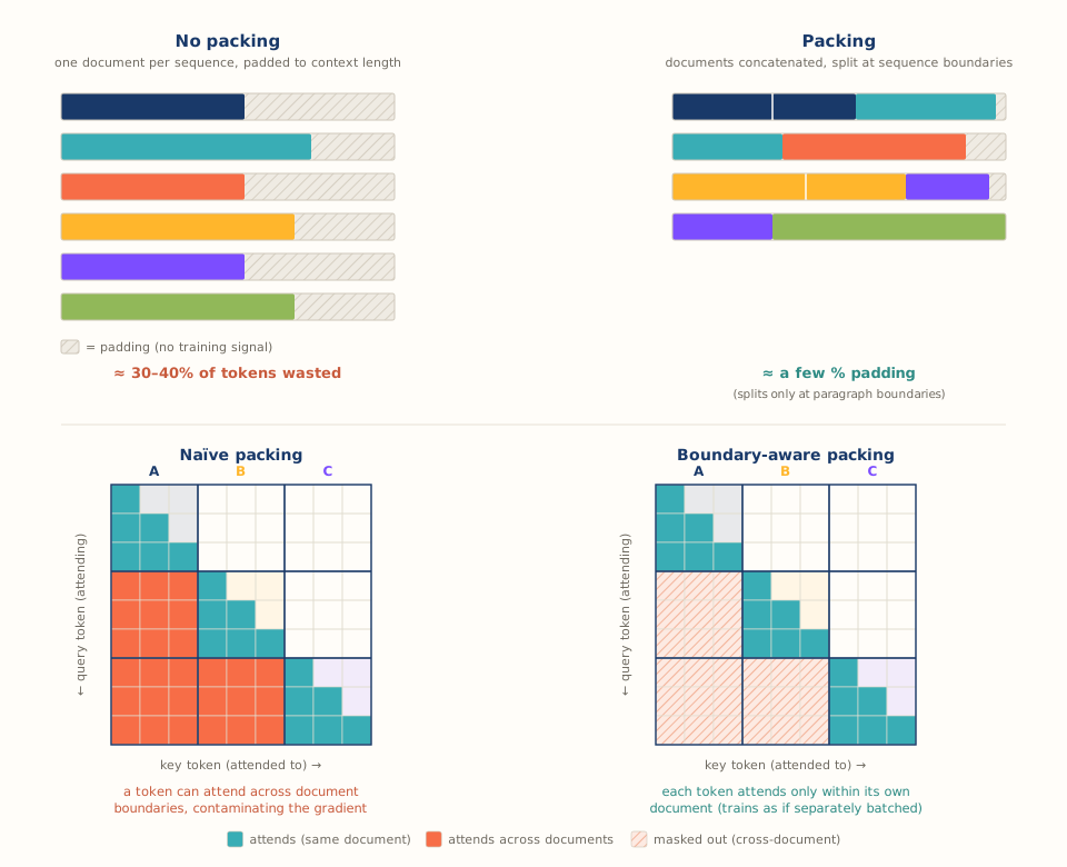
Top: six documents of different lengths. One document per sequence (left) leaves 30 - 40% of tokens as padding (note that for multi-node training, a global sequence length must be fixed); concatenating the documents (right) removes most of it, with a small residual if sequences are split only at paragraph or sentence boundaries. Bottom: the causal attention matrix over one packed sequence of three documents (A, B, C). Within-document attention (blue) is identical in both cases; naïve packing (left) additionally attends across document boundaries (gradient contamination and suboptimal memory scaling), while boundary-aware packing (right) masks those cross-document positions, so each document is treated as an individual sequence.
In GPU-hours this would mean the following. The public Qwen3.5-VL 122B-A10B SFT recipe runs at global batch size 36, with a maximum sequence length of 4,096, for 300k steps: roughly 44B training tokens, or about 2'100 GPU-hours on 48 H100s at 35% MFU. At a worst-case 40% padding waste, ~840 of those GPU-hours are spent processing padded positions that contribute no useful training signal. Scaling the same math up, a 100B-token run wastes around 1'900 GPU-hours per recipe ablation, and the 1T-token target wastes around 19'000. That's roughly $76K per run at typical H100 cloud pricing of around 4$/GPU-hour.
What did the model actually see?
One subtlety matters here specifically since the realized and planned data mixtures can deviate substantially: The planned mix is a list of sources with their target shares, a set of filter parameters, and a training schedule. However, what reaches the model might deviate substantially from this planned mix. We illustrate this with the figure below (left panel). A declared (sample level) recipe would contain 71% web-scale biomedical text data; however, after transformations and filters are applied, sequences have been packed, and bad or uninformative samples removed (think of corrupted images that previously weren’t caught), the true token level mixture looks quite different, with a sharply decreased share of the web scale text dataset. Further looking at the loss token share per dataset, the tension relaxes but still strongly differs from the declared mix.
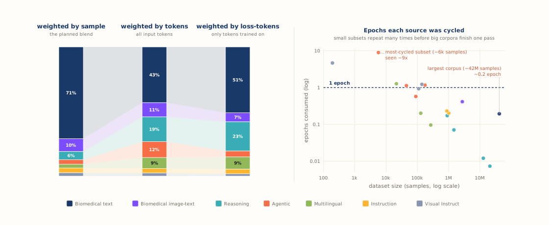
A real run (~20B tokens; sources anonymized), counted three ways. Left: the same realized data weighted by sample, by token, and by loss-token. By sample it matches the declared blend (71% biomedical text / 10% biomedical image-text / 19% skill additions); by token, biomedical text falls to 43% as token-dense skill data more than doubles its share; by loss-token (prompt, system, and image tokens masked out) biomedical text climbs back to 51%, while masked tool-use data collapses from 12% to 5%, far less than its token share suggests. Right: sources differ in size, so a small tool-use subset is cycled ~9 times before the largest corpus finishes a fifth of one pass.
Another aspect that is crucial to monitor is the number of times each dataset in the mix is seen. A first best judgement blend will be altered through the aforementioned dynamics and consequently we might be seeing the same samples more than intended. The right panel of the figure illustrates this, where a small tool-use dataset is heavily oversampled. The mechanism is as follows: While the dataset might have been correctly weighted by token share (tool-use data tends to come with fewer samples but very long sequences), many of the samples would exceed the context window of the initial stage of CPT already with the system message and user prompt, which depending on the training configuration may leave no tokens relevant for gradient calculation at all and thus are filtered on the fly. The resulting over-representation of the dataset in the mix requires a subsequent re-adjustment.
The cost of being wrong grows with run size. At the trillion-token scale we're working toward, a 1% drift in the realized mixture is 10B tokens of unintended training spent on the wrong distribution (about the entire budget of a respectable open research run). Our token-level observability stack ensures that any drift is visible at training time and not hidden in a silent performance drift in evaluation.
A trustworthy evaluation signal
Checkpoint validation is our main signal for whether the upstream work paid off, so it carries the same engineering investment as training and data.
Contamination is a sharper risk for us than for a research model. A research model is judged on a fixed, public benchmark set it can decontaminate against; our models are judged by users on clinical tasks we may not have anticipated. Therefore, we evaluate against both critical public benchmarks and internal private ones, and keep adding and revising them as the product surface grows. One uncaught test-set leak turns that signal into a misleading one.
Therefore, we deduplicate every training source against every active benchmark. Exact matching runs on every pair; we add the costly fuzzy and semantic passes where source and benchmark draw on shared material. Overlap on the rest is tracked as a tripwire, escalating a pair if it climbs above a threshold.
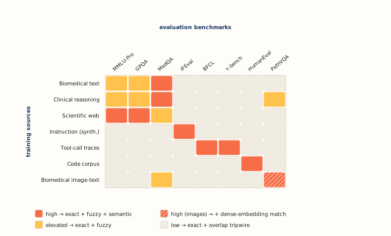
Leakage risk varies across (training source × benchmark) pairs, so we target the expensive matching rather than spread it evenly. Every pair is deduplicated by exact match; where a source and benchmark draw on shared material (high-risk pairs) we add the full fuzzy and semantic stack (dense-embedding matching for images). Overlap on the rest is tracked as a tripwire and escalated if it climbs. New sources and benchmarks are matched against everything active as they come online.
A trustworthy signal needs two things: a benchmark the model has not already seen, and a way to read why a score moved. For the first, we escalate the matcher, each step catching what the one before it cannot:
- Exact match. Verbatim copies fall out of a hash match, run on every (source × benchmark) pair.
- Fuzzy matching. Reformatted and reworded copies survive it: MinHash-LSH surfaces near-duplicates by Jaccard overlap4.
- Semantic matching. What survives fuzzy is caught by embeddings: a cosine pass over text5, and dense image embeddings with approximate nearest-neighbour search that flag a training image answering a benchmark question even when its pixels differ. Both carry a higher false-positive cost, so we reserve them for pairs where a source and benchmark share material, as illustrated in the figure.
For the second point, we store all generations and not just the score. We pull actual generations from each checkpoint and inspect a few of them by hand and with an LLM judge at scale, because a drop in a benchmark has many possible causes a single number hides. A common example is a drop in performance, where the model gives the right answer in the wrong format, so the failure is instruction following, not knowledge. A score alone cannot tell the two apart.
Conclusion and outlook
Every stage in this post acts on the same data mixture: the framework and packing deliver it, observability records what the model actually trained on, and decontaminated evaluation shows whether it worked. Each component is built to hold as runs scale, so moving from today's 100B-token runs to the trillion-token target on 100B+ MoE models means changing the configuration, not rewriting the stack. What remains is to compose them into a single loop.
That composition is what we are building toward in kaiko's AI Factory, a pipeline where evaluation results feed back into the recipe directly, the recipe as a versioned, structured artifact and the observability primitives from the preceding sections making each stage's output legible to the next. The orchestration already runs on Dagster, workloads are distributed via Ray, and Kubernetes provisions and schedules the resources. The components exist today (framework, loader, packing, decontamination, a trustworthy evaluation signal, an emerging recipe artifact). Composing them into a single closed loop is the work ahead, and the subject of a future deep dive.
None of these practices are novel on their own. The literature has assembled most of the pieces. What rarely makes it into a paper are the steps behind a headline: preempted and crashed runs, the mixture drifting from the recipe, or a dataset silently cycled nine times. With this article, we want to shed some light on what it takes to move toward the trillion-token frontier.