Every run explains itself

Summary
Training large multimodal models for clinical reasoning can involve hundreds of GPUs running for weeks. At that scale, small performance regressions are costly, and distributed failures can take hours to diagnose. This post describes two parts of our training infrastructure designed to address these problems:
- Performance diagnosis. A profiler captures a few steps in kernel-level detail and reduces the trace to a named bottleneck. A lightweight monitor tracks the full run, from model FLOPs utilization (MFU) to per-collective communication time, so regressions are visible as they happen.
- Operational reliability. A canary tests the allocated compute, network, and storage before and periodically during training. A health monitor records progress on every rank and combines evidence from a distributed failure into one report, identifying either a likely originating rank or a shared fault domain.
Introduction
Training large multimodal models for clinical reasoning means running jobs on hundreds of GPUs across dozens of nodes, for days, sometimes weeks. At that scale, performance depends on every part of the distributed system. Training is synchronous, so a slow GPU, network link, or input pipeline can hold back the entire job. The same clusters run a steady stream of smaller experiments, so slowdowns and failures affect both large training runs and how fast we can test new ideas.
Understanding why a run is slow requires visibility at different timescales. A profiler can explain a few steps in detail, but overhead and trace volume make continuous capture impractical. Dashboards track throughput and utilization over the full run but do not show where step time is lost. Cluster health checks can report that a node is available without revealing that a GPU is throttling, an interconnect is underperforming, or storage cannot keep up with the workload.
Failures create a different problem. An error on one rank (one GPU process) often causes communication timeouts on others, leaving many secondary errors but little indication of the original fault. Diagnosing the incident can require comparing worker and cluster logs, scheduler events, dashboards, and hardware telemetry across the allocation. By the time the investigation begins, the scheduler may have already torn the job down and removed the most useful local state. None of this is rare at scale. Meta reported an unexpected interruption roughly every three hours during the 54-day pretraining of Llama 3 405B1.
We built our own observability layer around a single principle: a run should explain itself. We record traces, timers, hardware counters, and per-rank heartbeats while the job is running and preserve them through teardown, so why a run is slow and why it failed is evident from what it recorded.
Two pillars, four instruments
To make that possible, we use four components, grouped under performance and operational reliability (Figure 1).
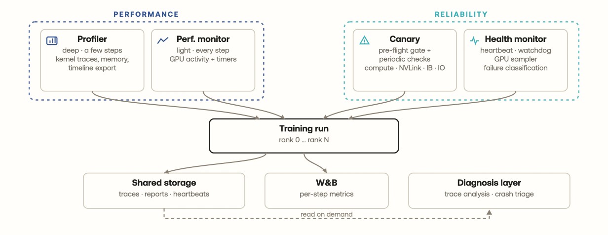
Figure 1: The four components, grouped into two pillars. Left (performance): a profiler for deep, occasional captures, paired with a lightweight monitor that runs the whole job. Right (operational reliability): a canary that benchmarks the assigned hardware before and during the run, paired with a health monitor that watches every rank. All four attach to the training run and write to shared storage and the experiment tracker, where one diagnosis layer reads them.
The profiler records a short window of kernel, memory, and communication activity in full detail. The performance monitor tracks throughput, framework timers, and GPU counters for the entire run, providing one summary line per logging interval.
The canary benchmarks compute, interconnect, and storage on the allocated nodes before training begins. It repeats a smaller set of checks during training. The health monitor keeps a heartbeat and a watchdog on every rank throughout. It performs a few cheap in-memory updates per step, enough to tell at any instant whether a rank is still making progress. It collects failure evidence the moment one stops.
The four are paired because neither kind is sufficient alone: profiling and full benchmarks are too heavy to leave on, while the continuous signals cannot explain what they detect. In practice, the monitor or canary notices a change, and the profiler or health monitor explains it. All four write their outputs to shared storage and the experiment tracker in formats the same analysis code reads through a single API, so after a slowdown or a crash the evidence is already in one place. Figure 2 shows when each component runs.
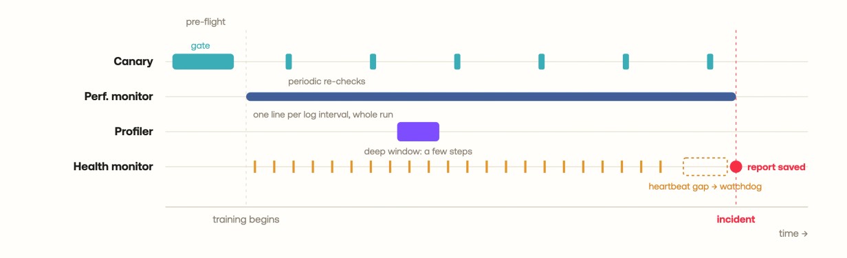
Figure 2: Time runs left to right across four lanes, one per component. The canary gates the start with a pre-flight check and re-checks periodically; the performance monitor emits one line every logging interval for the whole run; the profiler captures a short, deep window; the health monitor heartbeats continuously and, at the incident on the right, writes a report before the allocation is torn down.
Anatomy of a slow step
A useful profile should end with a diagnosis, for example: non-overlapped NCCL work accounts for a third of this step, making it communication-bound. Producing that diagnosis automatically is harder than collecting the trace. A few steps of a multi-node mixture-of-experts model generate hundreds of thousands of events across dozens of GPU streams.
We use the PyTorch profiler by default: it records a fixed set of steps and exports a Kineto trace, per-rank kernel summaries, a categorized memory timeline, and an allocator snapshot whose stack traces survive an out-of-memory crash. For system-level or individual-kernel analysis, we use Nsight Systems or Nsight Compute, with custom NVTX ranges marking the relevant model regions.
Each trace is parsed on the node where it was produced and reduced to a few kilobytes. This includes GPU busy and idle time, the compute/NCCL/memcpy split, the kernels consuming the most device time, and peak memory per device. This is the same reduction problem behind Meta's Holistic Trace Analysis2.
A priority-ordered classifier maps those measurements to a coarse bottleneck category:
- Launch-bound — high idle time and many short kernels: the CPU is not issuing GPU work quickly enough.
- Input-bound — high idle time with normal kernel durations: the input pipeline is not keeping up.
- Communication-bound — NCCL consumes a large share of
busy time; per-collective timings determine how much sits on the
critical path rather than overlapping compute. - Transfer-bound — host-device copies consume a large share of the step.
- Compute-bound — none of the previous conditions applies.
These labels describe the step as a whole. A compute-bound step can still contain kernels limited by memory bandwidth, occupancy, or instruction dependencies. Nsight Compute provides that finer distinction. Communication time also needs cross-rank context. If one rank, pipeline stage, or expert receives more work, faster ranks spend longer waiting in collectives, and an imbalance elsewhere ends up counted as NCCL time. We separate the two by comparing compute and input time across ranks.
The classifier always returns its supporting measurements, and its thresholds are versioned and tested so an engineer can inspect or override a verdict without reopening the full trace.
Figure 3 shows one of our training runs before and after acting on a communication-bound verdict. The optimized step is shorter, and its compute share rises because communication and idle time fall relative to the shorter total.
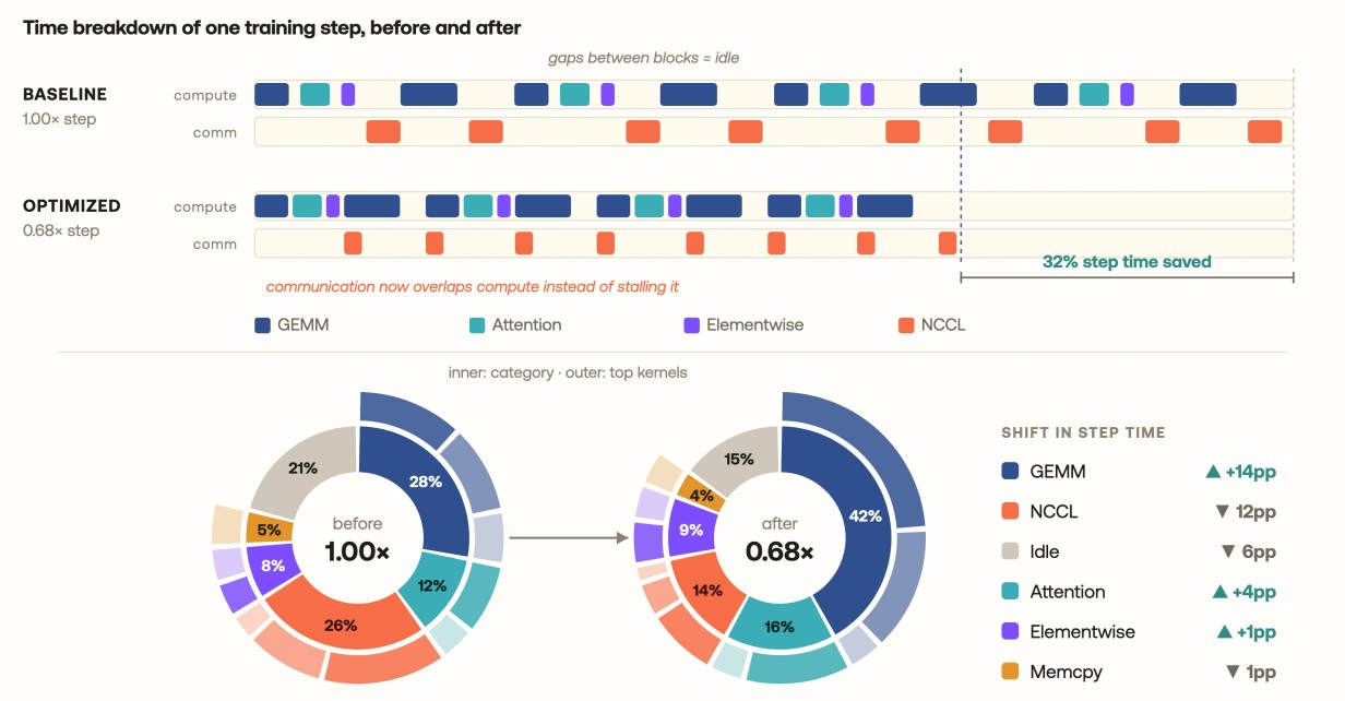
Figure 3: One training step before and after acting on a communication-bound verdict, here by overlapping communication with compute. Top: the step as two lanes, compute and communication; each block is a group of kernels, and the gaps between blocks are idle time. In the baseline, communication stalls compute; optimized, it runs underneath compute instead, so the step finishes ~32% sooner. Bottom: the same two steps as rings, inner ring by category and outer ring by the largest kernels within it. These are single operations such as one matmul or one all-reduce, showing which specific kernels dominate the category. Each is normalized to its own step so they show where time goes rather than absolute duration.
We use the verdict to choose the next experiment. Communication bottlenecks lead to overlap or collective changes. Launch bottlenecks lead to fusion or graph capture. Input bottlenecks lead to the loader and storage path. When an individual operation remains expensive, we write a Triton or CUDA replacement and keep it in an in-house kernel library that the training stack pulls from instead of the stock op. Every change is re-profiled before it is kept.
Monitoring performance over a full run
A profiler samples a few steps by design: depending on the configuration, profiling adds roughly 5–30% overhead, and on a healthy run most captured data is redundant. So we pair it with a lightweight performance monitor that runs for the full job. The key metric over that horizon is model FLOPs utilization (MFU)3: an MFU of 50% means the achieved model throughput is roughly half of the GPU’s theoretical peak at the training precision. We use it to track workload over time and compare related configurations. It is more informative than GPU utilization alone since a GPU can stay fully utilized while spending time on communication or inefficient kernels.
MFU on its own cannot explain a regression. To locate the cause, the monitor fuses hardware counters from DCGM (SM and tensor-core activity, occupancy, memory) with the framework's timers (compute, communication, pipeline bubbles, data loading) and adds timers where the framework is too coarse.
Communication is where those extra timers matter most. An NCCL call returns to the host almost immediately while the exchange runs asynchronously on the GPU's communication stream, so a host-side timer captures little more than the kernel launch. Instead, the monitor brackets each collective with CUDA events on its own stream and reads back the elapsed device time. This captures how long the exchange really took and how much overlapped with compute rather than stalling it. Tagged with its process group (data, pipeline, expert, or tensor parallel), this turns communication from one opaque bar into per-collective time attributed to the part of the parallel configuration that produced it.
The hardware is guilty until measured
A node can pass cluster health checks yet run below expected performance: a GPU throttling under sustained load, an NVLink or PCIe link operating below expected width, or a storage mount delivering insufficient throughput. Because each step includes synchronous collectives that all ranks must complete, the slowest affected rank can reduce throughput for the whole job4, and nothing crashes or reports unhealthy while this happens.
The canary tests the nodes and topology assigned to the run by executing inside the training process group itself. Before the first step, it benchmarks per-GPU compute throughput, intra-node and inter-node collective bandwidth, and storage read throughput, and records clocks, thermals, throttling state, and hardware error counters. Results are reported per rank, and the lowest-performing rank determines whether the allocation passes. A failed pre-flight check blocks training from starting, allowing the job to be rescheduled so a bad node costs minutes to reschedule around rather than days of degraded throughput.
During training, it periodically repeats a smaller set of checks. Measurements taken under load are usually lower than idle pre-flight results. Two mechanisms sit on top: hard thresholds relaxed to a fraction of the pre-flight value, which catch outright failure, and an exponentially weighted moving average of each measurement. This average flags sustained deviation from the pre-flight distribution and catches gradual degradation, such as a link losing bandwidth over hours, long before the relaxed threshold fires. Figure 4 shows one such event.
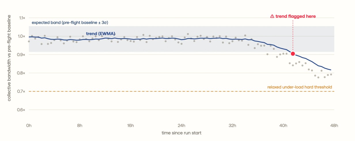
Figure 4: Each dot is a periodic in-flight measurement of collective bandwidth, as a fraction of the pre-flight baseline (vertical axis) over the course of the run (horizontal axis). Because individual samples are noisy, the canary tracks their exponentially weighted moving average (the trend line). As a link slowly degrades, that trend crosses its expected band and flags the problem hours before the measurement would trip the relaxed hard threshold; the gap between the two is the early warning.
When a run dies at 3am
Distributed failures produce secondary errors that often obscure the original fault. In an asymmetric failure, one rank fails first and the remaining ranks time out later in a collective. In a correlated failure, several ranks fail together because they share a host, switch, storage dependency, or scheduler event. In both cases the allocation may be torn down before the relevant local state is retained.
The health monitor runs on every rank. Background threads record the current step, phase, and timestamp, sample GPU state into a ring buffer, and run a progress watchdog. The training path performs a few in-memory updates and no synchronous I/O.
When a rank crashes, or the watchdog sees progress stop, the monitor collects every thread's stack, recent GPU state, PyTorch's NCCL flight-recorder entries, the other ranks' latest heartbeats, and the local exception, and writes them into one structured incident report on shared storage. A rule-based classifier labels the common cases: out of memory, software exception, data-pipeline stall, storage timeout, collective mismatch or deadlock, straggler, node failure.
Two real crashes show what this looks like in practice. One run died at step 62; the raw stack said only that a data-loader iterator had failed, and the report unwrapped the worker's traceback to the underlying stale file handle, so the cause was the shared filesystem briefly dropping its mounts mid-read. Another run died at step 2000 with an NCCL error in its logs; the report showed the CUDA allocations behind a collective failing because the GPU had run out of memory. The raw logs of the two runs look similar, and the reports separated them into a storage fault and an out-of-memory failure.
Cross-rank timing is most useful for asymmetric failures. The rank whose heartbeat stops first, carrying an exception the others do not share, is usually the source, and the timeouts that follow trace back to it. For correlated failures, the report groups affected ranks by shared host, switch, or dependency, since there may be no originating rank. In one incident, every rank reported a communication timeout, but one had stopped heartbeating about thirty seconds before the others inside the expert-routing all-to-all dispatch5. The ranks exchange data-dependent amounts of expert traffic and must first agree on the exchange sizes. Padding to a fixed expert capacity made the sizes static and removed the synchronization point where the run hung.
Runs that read their own reports
All of this was built for people first, but the same artifacts are exposed as tools over the Model Context Protocol so diagnosis can be invoked programmatically too. An agent can pull a crash report and apply the same odd-one-out triage, trigger the on-node trace analysis, and return the verdict with its evidence. It can also watch throughput and flag a sustained regression. The instruments supply the measurements, the agent summarizes them, and any action that costs cluster time still goes through a human. The practical effect is that routine questions no longer require an engineer to open a raw trace.
Conclusion and outlook
The tools presented in this post address two recurring ways a run wastes the hardware it holds: running below its capacity, and failing in a way that is slow to diagnose. The profiler and performance monitor show where step time goes and whether performance changes during a run. The canary verifies the assigned hardware before training and detects degradation while the job runs. The health monitor records per-rank progress and preserves enough evidence to distinguish an originating error from the failures that follow it.
Folding them into the closed loop of our AI Factory is the work ahead and the subject of a future post.