Inside the Medical AI Factory

Summary
Making a frontier model excel at clinical work takes thousands of experiments, some running on hundreds of GPUs for weeks. At that scale, model development has to work like a production line. The AI Factory is the platform we built to automate it, connecting diverse environments and workflows — from local development to distributed training — into a reproducible pipeline from source data to a post-trained model, while preserving the strict boundaries that medical data demands. This article introduces the AI Factory and shows how it accelerates research cycles, letting a small team develop frontier models for the clinic quickly and reliably.
Frontier models are strong generalists. In the AMA's 2026 survey, four in five US physicians reported using AI in their practice, most often to summarize research and draft documentation. But clinical work also demands skills not in the models' training data: operating the tools and systems clinicians work with, like navigating a gigapixel pathology slide to describe the findings.
At kaiko, we close that gap by taking open frontier models and training them for clinical use. That work runs from clinicians describing their workflows, through collecting or synthesizing training data, to integrating it into the training mix. Every change requires controlled experiments, run at more than one scale and across different training stages. Ideas are never in short supply, so the pace is set by how quickly they can be turned into experiments that can be trusted. Earlier articles described the models we built and how we train them at scale; this one focuses on the machinery that speeds up research cycles.
1. Enter the AI Factory
The AI Factory is the platform we built to make the experimentation loop fast and reliable. It turns a stream of changes into controlled experiments that can be trusted. The factory framing was inspired by Poolside's Model Factory.
Consider the following example: a new dataset has been transferred from a data partner, and we want to see whether it improves the model. Integrating the new dataset into training is rarely a single step. The data has to be validated, filtered, deduplicated, copied to the compute cluster, included in the training mix, and so on.
With the AI Factory, the whole cascade through data and training pipelines becomes a single change, versioned and reproducible (Figure 1). It can be a single pull request that declares the new dataset, plugs it into the existing pipeline, and adds it to the training mix. On merge, the platform takes over: it materializes the dataset while the CI builds and publishes the container image with the new training mix inside, and smoke tests the training pipeline overnight. The next training run automatically picks up the change, spins up a fresh cluster of GPU workers that find the dataset already waiting, and streams progress and results back to where it was started.
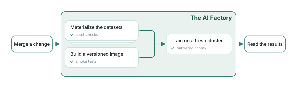
Figure 1: In the AI Factory, a single change can trigger the whole pipeline from source data to post-trained model. The platform materializes the datasets while the CI builds and publishes the image with the new training mix inside. The training run finds both waiting on a fresh cluster of GPU workers. Each step carries checks that can gate what follows.
Automating the trip from a change to its results enables running more experiments. But the goal of each experiment is to answer a specific question, which takes more than automation. To attribute an outcome to a change, everything else has to hold still, which requires reproducibility. The result of an ML experiment depends on the code, data, dependencies, and runtime environment, and any one of them drifting between two runs can be enough to change the resulting model. A run that cannot be trusted to reflect exactly one change can produce misleading conclusions. Reproducibility is the foundation for turning GPU-hours into durable answers.
The AI Factory's automation and reproducibility rest on three design principles:
- The image is the unit of change. Training code and its dependencies are baked into one container image, rebuilt and versioned automatically on every change. The image pins what runs.
- One path works everywhere. A file path resolves to the same data on a GPU cluster, in a development or production deployment, and on a laptop. What it returns depends on access, not on location.
- Every run gets its own cluster. A fresh cluster of GPU workers is created when a run starts and torn down when it ends. Each run gets a clean environment, isolated from all other runs.
Section 2 introduces the components that implement these principles, and describes how they preserve the boundaries that medical data demands. Section 3 shows how the factory speeds up research, making experiments controlled and repeatable, and catching failures before they burn GPU-hours.
2. A tour of the machinery
The AI Factory spans several environments. A change begins on a researcher's laptop and lands in a shared repository. From there, the data and training pipelines that pick it up are coordinated from the factory's control plane. The control plane is hosted on managed Kubernetes, while the training itself happens in separate GPU clusters. The change has to make that trip without quietly changing meaning. Wherever the job runs, the same code, dependencies, and data should produce the same result, even months later.
Three gaps sit along the route: the change has to be integrated into tracked pipelines, the job has to cross from one cluster to another, and the same data has to reach every environment. The AI Factory bridges each gap with a dedicated component.
2.1 The orchestrator
The first gap sits between locally developed code and tracked pipelines. A tracked pipeline records what it read, what it produced, and how to run it again. This record is what makes a run reproducible, and only a tracked pipeline keeps it.
We bridge this gap with Dagster, the factory's central orchestrator. It coordinates work without doing the heavy lifting. All pipelines run through Dagster, from downloading and pre-processing data to submitting training runs; it keeps track of what should exist, launches the work that produces it, and records every run.
Dagster's central abstraction is the asset: something that should exist (e.g., a dataset or model), paired with the code that produces it. Every asset declares which other assets it is built from, so together they form a directed graph that traces the lineage of everything the factory produces.
Steps like general-purpose pre-processing are no longer part of a training job. Each step becomes an asset, so the code sits next to the data it produces and the output takes a name and place in the graph. The output outlives the job that made it, ready for other pipelines to build on and easy for any colleague to find. A new dataset enters the graph as a single pull request that declares the source and every step downstream as assets. As an example, Figure 2 shows the resulting graph for a public dataset: one asset downloads the raw files, the next cleans them and normalizes the schema, a third splits the data into training, validation, and test sets, and a final step converts each split into a training-ready format.
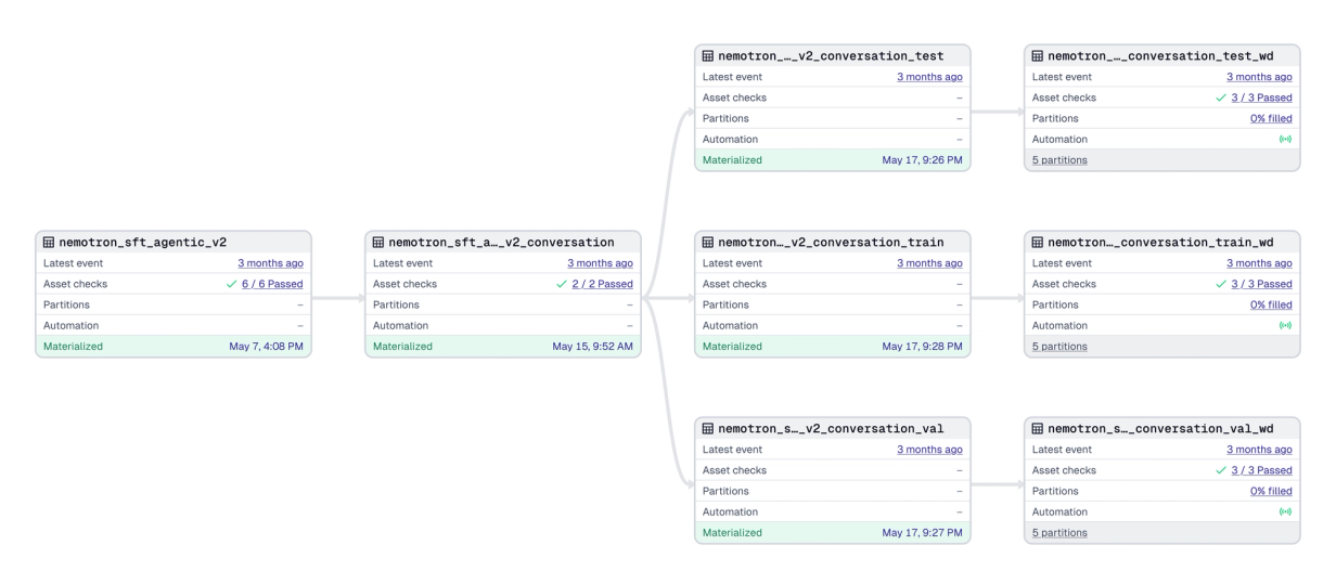
Figure 2: The lineage of a public dataset in the Dagster asset graph: from the raw source, through cleaning and splitting, to a training-ready format per split. Every step is a tracked asset that records its latest materialization. Asset checks can validate the output of each.
Assets carry checks: small tests that run every time the asset is rebuilt, asserting that the files, counts, and schema are as expected. A failed asset check can block everything downstream, providing cheap insurance against wasting hours of compute on a GPU cluster.
Not everything is an asset. Data is modeled as assets because a dataset has one current state worth tracking. In contrast, a Dagster job can model an experiment, which varies by settings and produces many outputs, like the checkpoints along the way. Schedules and sensors let the factory start work on its own, producing the same trace as any run started by hand.
Assets, jobs, checks, and schedules are all discovered from a single directory of definitions in our repository. The same directory loads on a laptop, in a development deployment, and in production. The pipeline a researcher runs locally is the same pipeline that runs in production. This orchestration underlies the automation and reproducibility that speed up the experimentation loop (Section 3).
2.2 Crossing clusters
The second gap sits at the boundary between clusters. While the control plane lives in one cloud, the heavy lifting happens in the GPU clusters of the compute plane. Every run has to cross that boundary, and the machinery we introduce in this section makes the crossing invisible. For the researcher, a run on hundreds of GPUs in another cluster is submitted like any other Dagster job and watched from the same user interface. Figure 3 traces the crossing end to end, from the run leaving Dagster, through the scheduler's queue, to the cluster created for it, and back.
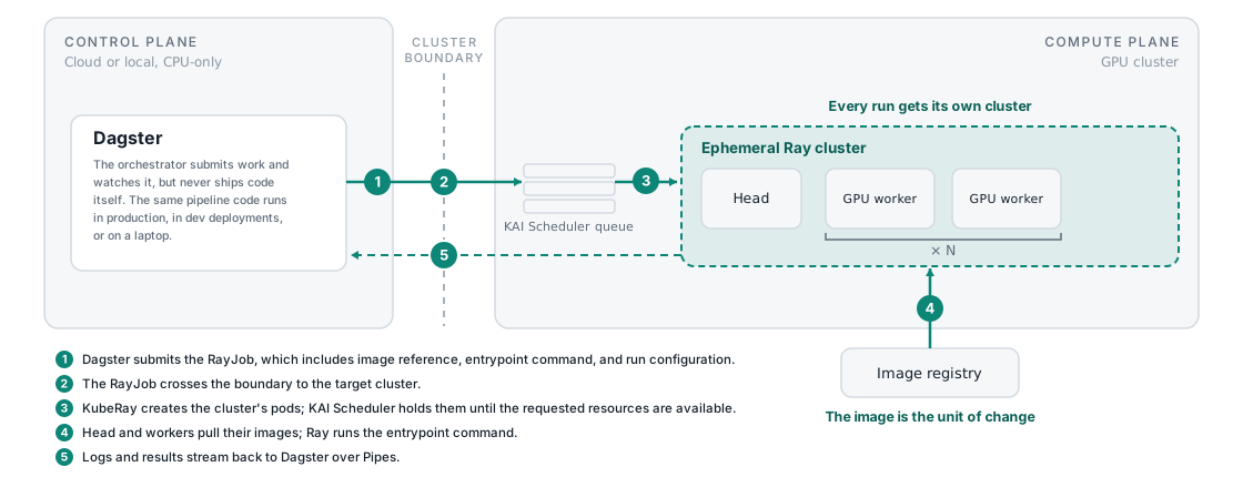
Figure 3: The path of one run across the two planes. Dagster submits a RayJob across the boundary, the scheduler admits it, an ephemeral Ray cluster pulls the image and runs the job, and logs and results stream back to Dagster.
Dagster stays on the control-plane side of the boundary and acts as a client. It submits the run and watches it, but never ships code to the workers. Instead of installing code and dependencies at job start, a step that can fail or drift on any run, the CI bakes them into a container image, rebuilt and versioned on every change. The training itself runs on Ray, a framework for distributing Python workloads across many machines, so what actually travels to the GPU cluster is a RayJob manifest that names the image, the entrypoint command, and the resources the run needs, such as the number of workers and GPUs.
Our Dagster–Ray integration carries the run across the boundary. It layers two pieces on the open-source dagster-ray library. First, a builder validates a given run config and turns it into the RayJob manifest. Second, a Dagster Pipes client launches the external job and streams its logs and results back to the orchestrator. The choice of which cluster the job lands on is one field in the run configuration. The same client resolves the address of the chosen cluster and handles the token authentication against it. The connection itself runs over Cilium ClusterMesh, which joins the two cluster networks so the orchestrator can reach the remote Ray endpoint as if it were a local service.
On the GPU cluster, KubeRay expands the manifest into a fresh Ray cluster, with a head node and GPU workers created for this run and torn down when it finishes. Every run gets its own cluster, so one run cannot interfere with another through a leftover process or a stale cache. And since every run names its own image, two experiments can run different software stacks side by side.
We use the KAI Scheduler, NVIDIA's open-source scheduler for GPU workloads, to decide when and where each run starts on the shared node pool. It follows written rules: a shared queue, explicit priorities, and preemption for lower-priority work. Gang scheduling places every worker of a job at once or makes the whole job wait, so a multi-node run never sits half-started, holding GPUs it cannot use. Once admitted, the pods pull the image from the registry, Ray runs the entrypoint command, and logs, events, and results stream back to Dagster over Pipes in real time.
For the researcher submitting the job in the Dagster UI, the machinery remains invisible. The run has made the trip across clouds, through a queue, into a cluster of its own, and streamed the results (or failure) back to the same interface.
2.3 Identical data everywhere
The third gap sits between two competing demands on the data. For training throughput, it belongs close to the compute, ideally in the same data center. But a dataset must also be the same wherever it is read: on the GPU cluster, in the orchestrator, and on a laptop. Copying data into each environment meets the first demand and undermines the second, because every copy is a chance for versions to drift.
We close this gap with Hammerspace, a layer that presents the storage across our sites as one file system. Instead of each environment keeping its own copy, they all mount one shared namespace. The orchestrator and GPU pods browse the same directory tree, and even a researcher working on their laptop can inspect the exact files a training run reads from the public tree. The tree mirrors the Dagster asset graph (e.g., Figure 2): a dataset's key in the orchestrator is its directory in the namespace, written once by the pipeline that materializes it and never copied anywhere by hand. One path works everywhere, so a dataset path copied from a run log resolves wherever it is pasted.
Underneath the shared namespace, a path says nothing about where the bytes live. Metadata nodes own the directory tree and decide where each file is stored, while data movers carry the bytes across sites when needed. To a job it all looks like ordinary network storage, mounted into its pods. Each Ray cluster starts with the directory tree in place, and reading it requires no library or special API, just a file path.
The namespace is identical across all environments, but the bytes stay local. At the GPU site, it is backed by fast storage in the same data center. Only background replication ever crosses the site link; every other environment reads the same files from its own local storage. Once a dataset has synced, a read never leaves the cluster. Freshly written data is the flip side: reads do not fail, since missing files are fetched on demand, but can be slow until the sync catches up.
Hammerspace ensures that even a modified or newly added dataset is already in place when a training run starts. The result is identical data everywhere, with fast local reads and no copies to drift. Meta co-developed a parallel NFS deployment with Hammerspace for the clusters that trained Llama 3, drawn by the same property: a change made anywhere becomes visible at once across all nodes and environments.
2.4 Access control by construction
The previous sections described how a change is carried across environments. When the cargo is sensitive medical data, access control is essential. Access rules are mostly enforced outside the AI Factory, while the factory ensures alignment. Everything it produces stays within those rules by construction.
The alignment rests on two properties of every asset: its path and the identity that wrote it. The first segment of every asset key is public or private, and because the key corresponds to the storage path, the classification travels with the data. The private tree is reachable only by the pipelines and projects that own the data. In the trees the factory manages, write access belongs to pipeline identities, so datasets there are, by construction, produced by version-controlled code that has been reviewed and tested.
The most sensitive data never reaches the factory at all. Incoming data that may contain personal information lands in a restricted zone outside the shared namespace. Only pseudonymized data leaves that zone, crossing into the private tree, where the factory can pick it up.
One piece of enforcement does live in the factory's code: pipelines derive the classification of an output from the classification of their inputs and refuse a mismatch, so a private dataset cannot end up in the public tree through a wrong prefix. Nobody has to remember which data is sensitive. Reads are decided by the path, writes by identity, wherever the job runs.
3. Speeding up research
The AI Factory carries a change from a laptop into tracked pipelines, across cluster boundaries, and onto machines that already have the data waiting, with logs and results streaming back. This section shows what that machinery enables: experiments that are controlled and repeatable, and checks that can catch broken data, faulty images, and flaky hardware before they hit a production run.
3.1 One change at a time
Suppose an experiment shows a curve that looks off compared to a baseline. Is it a side effect of the intended change, or something else that changed between the two runs? The code is usually version-controlled and easy to bisect. But ML experiments also depend on factors that can change silently between two runs, such as the data and code dependencies, which can alter training dynamics and hence the resulting model. In the worst case, hours go into retracing old runs, turning the day into a reproducibility quest.
Repeatable experiments require pinning four moving parts: code, data, dependencies, and runtime environment. Following the principle that the training image is the unit of change (Section 2.2), code and dependencies, including the GPU libraries, arrive pinned inside the image, which the CI rebuilds whenever either moves and bumps its version in the projects that use it. Additional run configuration, which can include hundreds of hyperparameters, travels separately and is recorded with the run in the orchestrator. A dataset does not have to be tracked separately from its sources, since its lineage records which inputs and code produced it. Together, these mechanisms pin all four moving parts, and any past run can be re-executed with one click in the Dagster UI.
Besides reproducibility, versioning every input makes it easy to undo changes and to isolate the effect of each. Any change can be rolled back atomically by pointing at an older version of the code or data. To find the root cause of an unexpected result, like the suspicious curve from our previous example, we can vary each part individually. Changes that span multiple parts can be combined in a single pull request. Datasets are declared in the same repository as the code that consumes them, so one rebuild pins both jointly. Even state that does not exist yet, like a dataset declared but not yet materialized, arrives pinned at the same version as the code that will use it.
The differences between a run and its baseline are no longer a mystery but a finite list of candidates. The remaining variation comes from nondeterministic kernels and communication order, not from a silent change. Finding what changed becomes less of a quest and more of a controlled experiment, conducted one change at a time.
3.2 Trust but verify
Reproducibility establishes trust, but only after the fact. A failed run still has to be debugged and re-run. The factory also verifies ahead of time, checking data, training images, and cluster hardware before a fault can hit a production run.
The data side is handled by asset checks (Section 2.1), which we can now see in action. A check runs against the dataset an asset produces and asserts one property: whether the schema is the one the next stage expects, the required columns are present, the row counts fall in range, or the files are intact. What makes a check more than a warning is that it can be blocking. A failure stops everything downstream, so a broken dataset never becomes an input to training. Figure 4 shows the execution history for one dataset's checks, with a schema check that failed on two earlier runs and passed on the most recent. Those earlier failures are the mechanism doing its work.
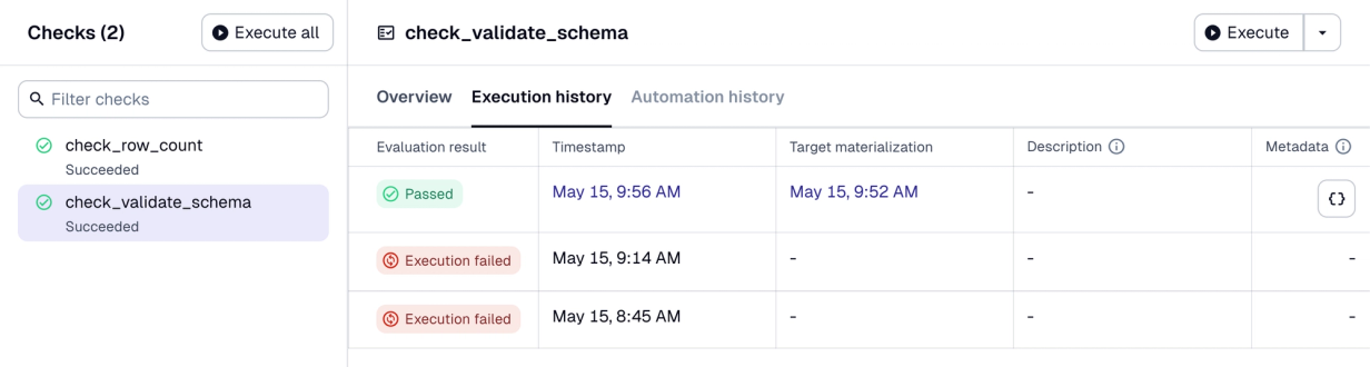
Figure 4: Execution history for a dataset's asset checks in the Dagster UI. Both checks succeed on the latest run. On two earlier runs the schema check failed and stopped everything downstream instead of letting bad data through.
Checking the data is not enough, because the training image itself can break in ways ordinary CI tests cannot catch. Some faults surface only on GPU hardware, when the image meets the driver and the workers connect across nodes. Nightly smoke tests exercise each new image end to end with short training runs, so a packaging or dependency fault shows up on a cheap overnight test rather than crashing a production run the next morning. The schedule is designed not to waste compute: an image that already has a green smoke test is skipped, so each image is verified exactly once. Figure 5 shows this in the schedule's tick history. A night after an image change requests one run, and a night without changes requests none.
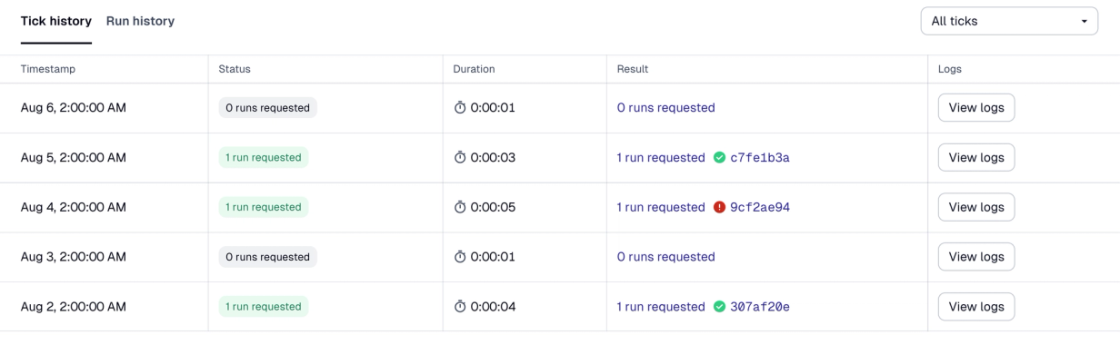
Figure 5: Tick history for a nightly smoke schedule in the Dagster UI. A new image requests a short end-to-end training run, which can pass or fail. An unchanged image requests zero runs, so each image is verified exactly once.
The last piece to check is the hardware itself. On a large-scale training run that uses hundreds of GPUs over days or weeks, a single flaky GPU or a degraded link can waste hundreds of GPU-hours. Every hour, a scheduled probe measures the bandwidth between pairs of idle GPU nodes, preemptible below training priority so it never delays a real run. Training runs also carry a canary, which benchmarks the assigned GPUs, NVLink, and InfiniBand fabric before and during training, as described in our previous article.
A broken dataset stops at its check, a faulty image fails its smoke test overnight, and a flaky GPU surfaces before training starts. These checks change what researchers spend the day on and establish trust in the underlying infrastructure.
4. Beyond training
Nothing in the AI Factory is specific to training. The same system can automate any workload that has to move reliably across environments. Automated evaluations can score every new checkpoint once a sensor detects it. Rejection sampling can turn model outputs into new training data, declared and versioned like any other asset. Batch inference over an entire archive can run as a downstream job, reading the trained model's weights directly from the shared namespace. Every workload runs on the same machinery, and the target cluster becomes just another field in the run configuration, a choice we plan to automate so each run lands where GPU capacity is available.
No honest tour of the machinery ends without a word about the running costs. Every component needs maintenance, and faces a redesign when demands change. The image that pins everything is rebuilt on every change, however small, which requires fast builds. The shared namespace keeps data identical everywhere, but serves freshly written data slowly until a sync catches up. A fresh cluster per run adds minutes of startup, negligible for a long training run but real overhead for a quick experiment. And the factory itself requires continuous maintenance and coordination between platform and research teams. So far, the running costs have been worth it. The factory carries hundreds of jobs a month, from dataset materializations to nightly smoke tests, each traceable to the inputs and code that produced it.
With the experimentation loop running on the AI Factory, the hours saved through automation and reproducibility go into improving the model. The principles that make it work are few: the image is the unit of change, one path works everywhere, and every run gets its own cluster. That foundation lets a small team develop frontier models for the clinic quickly and reliably, within the boundaries that medical data demands.
The models and methods described are research prototypes and have not been approved or cleared as medical devices. They are not intended for clinical diagnosis or patient care.